Introduction

The Naïve Bayes classification is based on Bayesian Theorem and is particularly suited when the dimensionality of the inputs is high. Despite its simplicity, Naïve Bayes can often outperform more sophisticated classification methods.

The Naïve Bayes probabilistic Model

Abstractly, the probability model for a classifier is a conditional model:

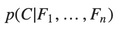
Over a dependent class variable C with a small number of outcomes or classes, conditional on several feature variables F₁ though F_n. The problem is that if the number of feature n is large or when a feature can take on a large number of values, then basing such a model on probability table is infeasible. We therefore reformulate the model to make it more tractable.

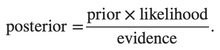
Using Bayes’ theorem, we write:

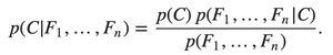
In plain English the above equation can be written as:

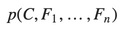
In practice we are only interested in the numerator of that fraction, since the denominator does not depend on C and the values of the features F_i are given, so that the denominator is effectively constant. The numerator is equivalent to the joint probability model (See Bayes theorem):

which can be rewritten as follows, using repeated applications of the definition of conditional probability:

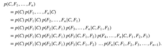
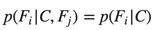
Now the “naïve” conditional independence assumptions come into play: assume that each feature F_i is conditionally independent of every other feature F_j for j≠i. For example, j≠i, k, l. the assumption means that:

So the joint model can be expressed as:

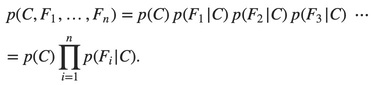
This means that under the above independence assumptions, the conditional distribution over the class variable C can be expressed like this:

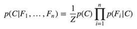
Where Z (the evidence) is a scaling factor dependent only on F₁,…,F_n

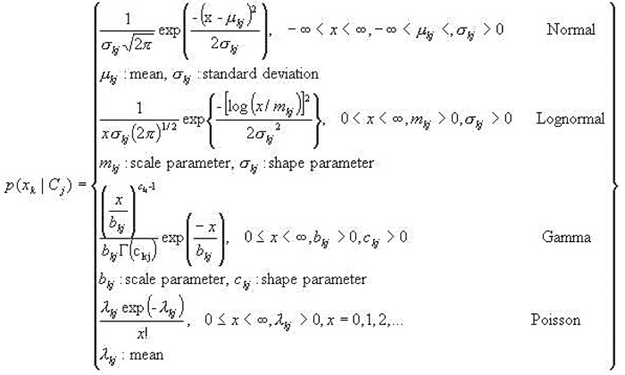
Naïve Bayes can be modelled in several different ways including Normal, Lognormal, Gamma and Poisson density function.

Example

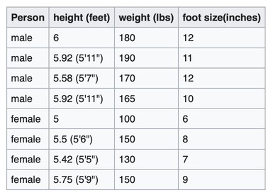
Problem: Using the following training set, classify whether a given person is a male or a female, based on the provided specifications. The known criterias are: height, weight, and foot size.

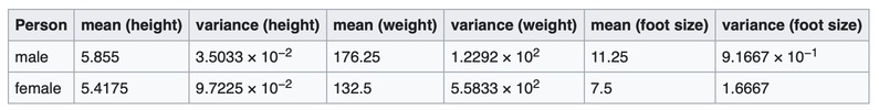
The classifier created from the above training data, using a Gaussian Distribution Assumption, would be:

Then, there is a sample to be classified as “male” or “female”:

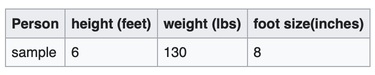
Our goal is to determine the greater posterior, “male” or “female”.

For the classification as “male” the posterior is given by:

For the classification as “female” the posterior is given by:

Next, the evidence may be calculated:

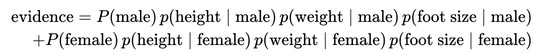
However, in this case the evidence is a constant. Therefore, both posteriors are scaled equally. That's why it can be ignored, since it doesn't affect classification.

Let's continue to calculate the probability distribution for the sex of the sample data:

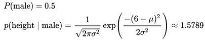
where and 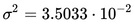are the parameters of normal distribution which have been previously determined from the training set. Note that a value greater than 1 is OK here – it is a probability density rather than a probability, because height is a continuous variable.

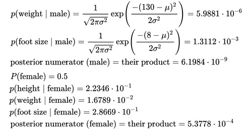
Since posterior numerator is greater in the female case, we predict the sample is female.

 

References & Resources

• Wikipedia
• Bindi Chen, the First Year Transfer Report - Progressing for the Degree of Doctor of Philosophy.