Scatter Plot

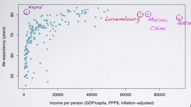
A common tool for visualizing the relationship between two numerical variables is a scatter plot. To identify the explanatory variable in a pair of variables, we identify which of the two is suspected of effecting the other and plan an appropriate analysis.

Since we might suspect that the economic wealth of a country might affect the average life expectancy of its people, we have set up our analysis with income as the explanatory and life expectancy as the response variable. Generally in scatterplot, we place the explanatory variable on the x-axis and the response variable on the y-axis.

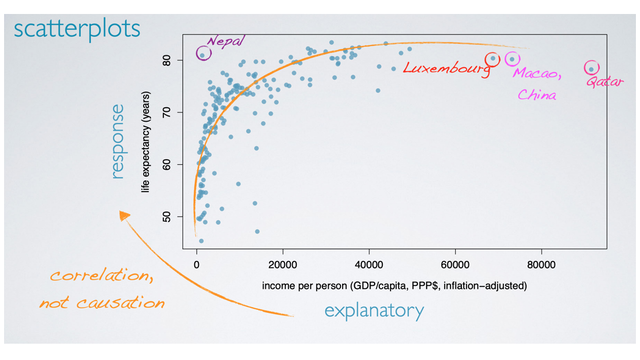
Since these data are observational and do not come from a randomized controlled experiment. We know that we can only talk about correlation, and not causation between the two variables. In order to see the nature of the relationship between these two variables, the best way to answer this question is to visualize a line or a curve going through the clot of the data. So here, we have drawn a curve that first shows a positive increase in life expectancy as income increases, then the relationship levels off (Such that countries with income levels above a certain point still have roughly 80-85 years of average life expectancy).

Evaluating the Relationship

When evaluate the relationship between two numerical variables, we should make sure to examine the direction of the relationship.

• Positive: Is it increaseing?
• Negative: Or decreasing?

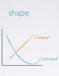
The shape of the relationship:

• Is it linear;
• Or non-linear;

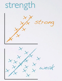
The strength of the relationship:

• Strong indicated by little scatter?
• Or weak, indicated by lots of scatter?

Any potential outliers? These can be individual observations, or a group of observations. Its always a good idea to investigate these points carefully to make sure they're not data entry errors.

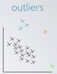
Let's take a closer look at those outliers we identified earlier. Some of them have pretty high income levels, Luxemburg a rich country with a small population enhance the high income per person level. Macau, a special administrative region in China, and Qatar, a country with a small population and lots of oil. Another potential outlier is Nepal, where the life expectancy is considerably higher than what would be expected for the low income level, compared to others. These are countries that we would indeed expect to behave differently than the majority of countries, so it's not surprising that they stand out from the rest.

One naive way of dealing with outliers in data analysis is to immediately exclude them, but we're calling that approach naive because it's often not the right approach. This is a good example of when the outliers might be very interesting cases. And handling them will take careful consideration of the research question and other associated variables.

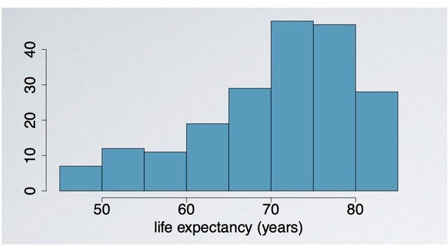
Histogram

One good way of visualizing the distribution of a numerical variable is a histogram. In a histogram, data are binned into intervals and heights of the bars represent the number of cases that fall into each interval.

• Provides a view of the data density.
• Especially useful for describing the shape of the distribution.

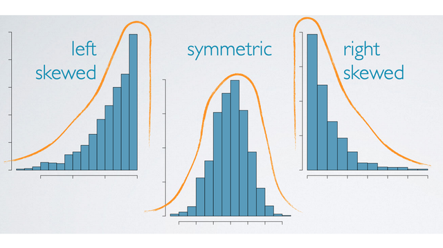
Skewness

Distributions are skewed to the side of the long tail.

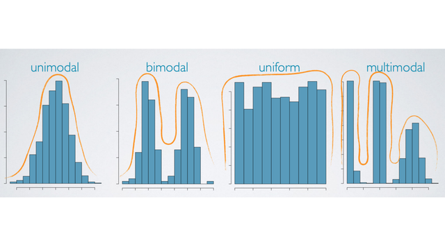
Modality

Prominent peaks determine modality

• A distribution might be unimodal with one prominent peak.
• Bimodal with two prominent peaks.
• Uniform with no prominent peaks,
• Multimodal is what we call a distribution when it has more than two prominent peaks.

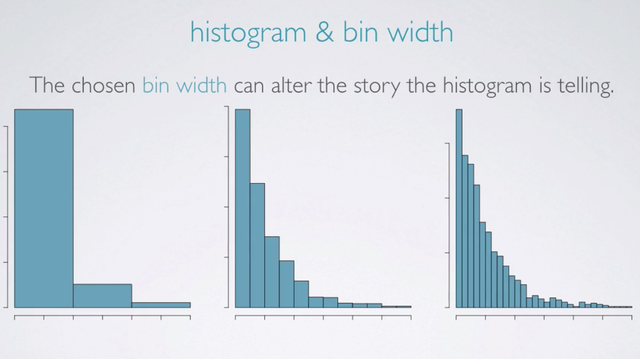
Histogram & bin width

We should also note that the chosen bin width of a histogram can alter the story the histogram is telling. When the bin width is too wide, we might lose interesting details. On the other hand, when the bin width is too narrow, it might be difficult to get an overall picture of the distribution. The ideal bin width depends on the data you're working with, so you should try playing with it until you're satisfied with the visualization.

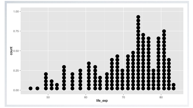
Dot Plot

Another technique for visualizing such data is a dot plot.

• A dot plot is useful especially when individual values are of interest.
• However, as the sample size increases, the dot plot may get too busy.

Box Plot

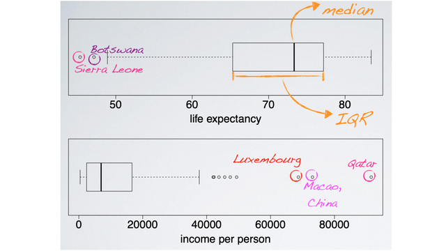
Yet another visualization technique, that is especially useful for highlighting outliers, is a box plot. A box plot also readily displays the median, the midpoint of the distribution. The thick line inside the box, and the interquartile range, the width of the box.

According to the top box plot, the median life expectancy is roughly 73 years old. And the middle 50% of countries have average life expectancies between roughly 65 and 77 years old. In addition, countries with life expectancies below, below roughly 48 years old are considered to have unusually low average life expectancies.

A box plot of the income distribution shows the same right skewed distribution we have identified before. And the outlying countries with unusually high income per person levels, stand out in this visualization as well.

The following attributes can be determined from a boxplot:

• Skewness;
• Outliers;
• Minimum and Maximum;

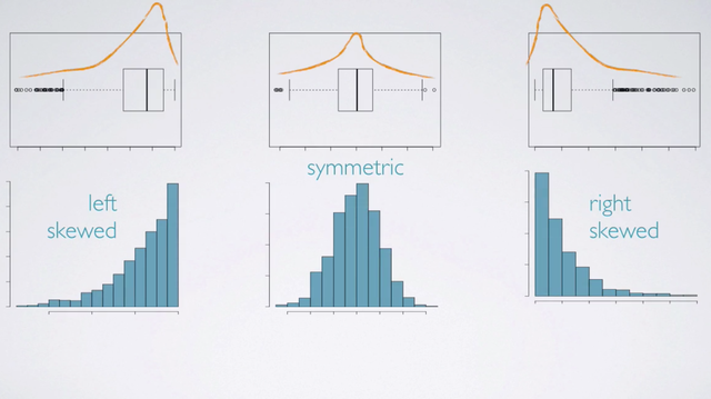
One way of determining the skewness of a distribution from a box plot, is to imagine what the histogram would look like. In other words, where the center of the distribution will be relative to the task. We know that the data can only span out to the edges of the box plot. And, that the center will be somewhere closer to the median. And then, we can connect the dots to figure out where the longer tail is going to be. Here, we have a left skewed distribution with a longer tail on the negative side. With the symmetric distribution the center is going to be in the middle and the tails will be roughly symmetric on both sides. And on the right skewed distribution the center is going to closer to the lower edge and the longer tail is going to span out on the positive side.

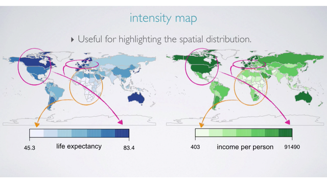
Intensity Map

For certain types of data, it might be useful to view the spacial distribution. These displays reveal trends in the data that many others did not. For example, we can see that both income and life expectancy are lower in Africa, but higher in North America and Europe.

References & Resources

• N/A