Introduction

The hierarchical clustering is a method of cluster analysis which seeks to build a hierachy of clusters. Strategies for hierachical clustering generally fall into two types:

• Agglomerative: This is a "bottom up" approach: each observation starts in its own cluster, an pairs of clusters are merged as one moves up the hierarchy.
• Divisive: This is a "top down" approach: all observations start in one cluster, and spilts are performed recursively as one moves down the hierarchy.

Both this algorithm are exactly reverse of each other. Here, we will be covering Algomerative Hierarchical clustering algorithm in detail.

Agglomerative Hierarchical clustering

This algorithm works by grouping the data one by one on the basis of the nearest distance measure of all the pairwise distance between the data point. Again distance between the data point is recalculated but which distance to consider when the groups has been formed? For this there are many available methods. Some of them are:

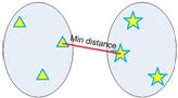
• Single-nearest distance or single linkage: minimum distance criterion.

  

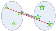
• Complete-farthest distance or complete linkage: maximum distance criterion.

  

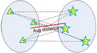
• Average-average distance or average linkage: average distance criterion.

  

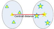
• Centroid distance.

  

• Ward's method - sum of squared euclidean distance is minimised.

Let  X = {x₁, x₂, x₃, ..., x_n} be the set of data points.

1. Begin with the disjoint clustering having level L(0) = 0 and sequence number m = 0.
2. Find the least distance pair of clusters in the current clustering, say pair (r), (s), according to d[(r),(s)] = min d[(i),(j)]   where the minimum is over all pairs of clusters in the current clustering.
3. Increment the sequence number: m = m +1.Merge clusters (r) and (s) into a single cluster to form the next clustering   m. Set the level of this clustering to L(m) = d[(r),(s)].
4. Update the distance matrix, D, by deleting the rows and columns corresponding to clusters (r) and (s) and adding a row and column corresponding to the newly formed cluster. The distance between the new cluster, denoted (r,s) and old cluster(k) is defined in this way: d[(k), (r,s)] = min (d[(k),(r)], d[(k),(s)]).
   
5. If all the data points are in one cluster then stop, else repeat from step 2).

Divisive Hierarchical clustering - It is just the reverse of Agglomerative Hierarchical approach.

Advantages and Disadvantages

Advantages

• No apriori information about the number of clusters required.
• Easy to implement and gives best result in some cases.

Disadvantages

• Algorithm can never undo what was done previously.
• Time complexity of at least O(n²log n) is required, where ‘n’ is the number of data points.
• Based on the type of distance matrix chosen for merging different algorithms can suffer with one or more of the following:
  •     i) Sensitivity to noise and outliers;
  •     ii) Breaking large clusters;
  •     iii) Difficulty handling different sized clusters and convex shapes;
• No objective function is directly minimized
• Sometimes it is difficult to identify the correct number of clusters by the dendogram.

Numerical Example

Here is a simple numerical example to explain the Agglomerative Hierarchical clustering.

References & Resources

• https://sites.google.com/site/dataclusteringalgorithms/hierarchical-clustering-algorithm
• http://en.wikipedia.org/wiki/Cluster_analysis