Real Number
Introduction
A matrix is a rectangular array of entries of elements, which can be variables, constants, functions, etc. A matrix is denoted by an uppercase letter, sometimes with a subscript which denotes the number of rows by the number columns in the matrix. For example, Am×n denotes a matrix with the name A, which has m rows and n columns. The entries in a matrix are denoted by the name of the matrix in lowercase, with subscripts which identify which row and column the entry is from. The entries in our above example would be denoted in the form aij, which would mean that the entry is in row i, column j. For example, an entry denoted as a23 would be in the second row, in the third column (counting from the upper left, of course) The entries in the matrix are usually enclosed in rounded brackets, althrough they may also be enclosed in square brackets. The following are examples of matrices:
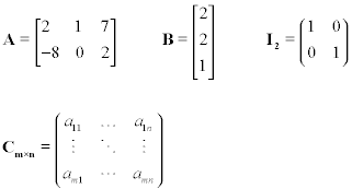
There are some special types of matrices. A square matrix has the same number of rows as columns, and is usually denoted Anxn. A diagonal matrix is a square matrix with entries only along the diagonal, with all others being zero. A diagonal matrix whose diagonal entries are all 1 is called an identity matrix. The identity matrix is denoted In, or simply I. The zero matrix Om×n is an matrix with m rows and n columns of all zeroes.
Given two matrices A and B, they are considered equal (A=B) if they are the same size, with the exact same entries in the same locations in the matrices.
Matrix Operations
Addition
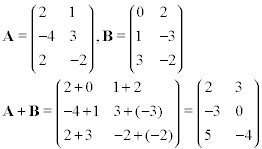
Addition of matrices is very similar to addition of vectors. In fact, a vector can generally be considered as a one column matrix, with n rows corresponding to the n dimensions of the vector. In order to add matrices, they must be the same size, that is, they must have an equal number of rows, and an equal number of columns. We then add matching elements as shown below,
Matrix addition has the following properties:
- A + B = B + A (commutative)
- A + (B + C) = (A + B) + C (associative)
Scalar Multiplication
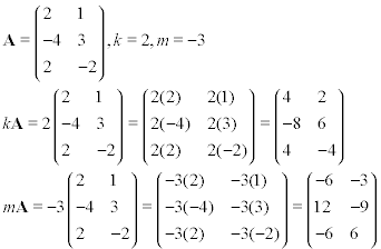
Scalar multiplication of matrices is also similar to scalar multiplication of vectors. The scalar is multiplied by each element of the matrix, giving us a new matrix of the same size. Examples are shown below,
Scalar multiplication has the following properties:
- c(A + B) = cA + cB (distributive), where c is a scalar
- (c + d)A = cA + dA (distributive), where c, d are scalars
- c(dA) = (cd)A
Matrix subtraction, similar to vector subtraction, can be performed by multiplying the matrix to be subtracted by the scalar -1, and then adding it. So, A - B = A + (-B) = (-B) + A. So like adding matrices, subtracting matrices requires them to be the same size, and then operating on the elements of the matrices.
Matrix Multiplication
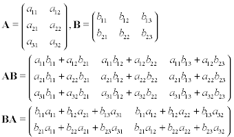
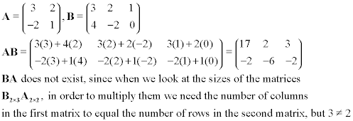
Two matrices can also be multiplied to find their product. In order to multiply two matrices, the number of columns in the first matrix must equal the number of rows in the second matrix. So if we have A2×3 and B3×4, then the product AB exists, while the product BA does not. This is one of the most important things to remember about matrix multiplication. Matrix multiplication is not commutative. That is, AB ≠ BA. Even when both products exist, they do not have to be (and are not usually) equal. Additional properties of matrix multiplication are shown below.
Matrix multiplication involves multiplying entries along the rows of the first matrix with entries along the columns of the second matrix. For example, to find the entry in the first row and first column of the product, AB, we would take entries from the first row of A with the first column from B. We take the first entry in that row, and multiply (regular multiplication of real numbers) it with the first entry in the column in the second matrix. We do that with each entry in the row/column, and add them together. So, entry abij = ai1b1j + ai2b2j + ... + aimbmj. This seems complicated, but it is fairly easy to see visually. We continue this process for each entry in the product matrix, multiplying respective rows in A by columns in B. So, if the size of A is m×n, and the size of B is n×p, then the size of the product AB is m×p. We show this process below:
We now show some properties of matrix multiplication, followed by a few examples:
- A(BC) = (AB)C (associative)
- A(B + C) = AB + AC (left distributive)
- (A + B)C = AC + BC (right distributive)
- k(AB) = (kA)B = A(kB), where k is a scalar
- AB ≠ BA (not commutative)
Matrix multiplication can also be written in exponent form. This requires that we have a square matrix. Like real number multiplication and exponents, An means that we multiply A together n times. So A2 = AA, A5 = AAAAA, and so on. We should note, however, that unlike real number multiplication, A2 = 0 does not imply that A = 0. The same is true for higher exponents.
Linear Combinations/Linear Independence of Matrices
Similar to the case with vectors, we can have linear combinations of matrices. In order to have linear combination of matrices, they must be the same size to allow for addition and subtraction. If a matrix A is a linear combination of matrices B and C, then there exist scalars j, k such that A = jB + kC. A set of matrices is said to be linearly dependent if any one of them can be expressed as the linear combination of the others. Equivalently, they are linearly dependent if there exists a linear combination of the matrices in the set using nonzero scalars which gives the zero matrix. Otherwise, the matrices are linearly independent.
Transpose of a Matrix
The transpose of a matrix A, denoted AT, is obtained by swapping rows for columns and vice versa in A. So the rows of A become the columns, and the columns become the rows. An example is shown below.
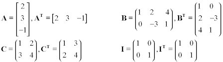
A square matrix is called symmetric if AT = A. Some properties of the transpose are:
- (AT)T = A
- (A + B)T = AT + BT
- (kA)T = k(AT), where k is a scalar
- (AB)T = BTAT
- (Ar)T = (AT)r, where r is a nonnegative integer
Please note the following theorems. The first is proved in the text, the second is proved in the sample problems for this section:
Theorem: If A is a square matrix, A + AT is symmetric
Theorem: For any matrix A, AAT and ATA are symmetric.
Inverse of a Matrix
Similar to the way that a real number multiplied by its reciprocal fraction gives us 1, we can sometimes get an inverse to a square matrix, so when a square matrix A is multiplied by its inverse denoted A-1, we get the identity matrix I.
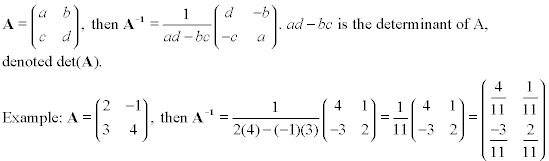
Please note that only square matrices can be inverted, and only some of those that meet a certain property.That certain property is that the determinant of the matrix must be nonzero. Determinants are explained more in the here (Gauss-Jordan Method of Finding the Inverse), but for 2x2 matrices, determinants and inverses are easy to find.
The inverse (if it exists) has the following properties:
- AA-1 = A-1A = I
- If A is invertible, A-1 is unique.
- (A-1)-1 = A
- (cA)-1 = (1/c)A-1, where c is a nonzero scalar
- (AB)-1 = B-1A-1, where A, B are the same size
- (AT)-1 = (A-1)T
- (An)-1 = (A-1)n, where n is a nonnegative integer
- A-n = (A-1)n = (An)-1, where n is a positive integer
We can easily find the inverse (if it exists) of a 2x2 matrix using the following formula:
Using the idea of inverses, we can use it to solve systems. Let A be a square coefficient matrix (size n×n) of a system of linear equations. Then if A is invertible, the system Ax = b has a unique solution by multiplying both sides of the equation by A-1, that is, x = A-1b, where b is a vector in Rn.
Elementary matrices
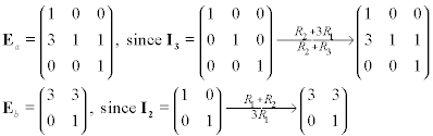
Elementary matrices are square matrices that can be obtained from the identity matrix by performing elementary row operations, for example, each of these is an elementary matrix:
Elementary matrices are always invertible, and their inverse is of the same form. Also, if E is an elementary matrix obtained by performing an elementary row operation on I, then the product EA, where the number of rows in n is the same the number of rows and columns of E, gives the same result as performing that elementary row operation on A. Finally, we can state the following theorem from the text (where you can also find the proof):
The fundamental theorem of invertible matrices, version 1:
Where A is a square matrix of size n×n, the following are equivalent:
- A is invertible
- Ax = b has a unique solution for every b in Rn
- Ax = 0 has only the trivial solution
- rref(A) = I
- A can be expressed as the product of elementary matrices.
References & Resources
- http://algebra.nipissingu.ca/tutorials/matrices.html
Latest Post
- Dependency injection
- Directives and Pipes
- Data binding
- HTTP Get vs. Post
- Node.js is everywhere
- MongoDB root user
- Combine JavaScript and CSS
- Inline Small JavaScript and CSS
- Minify JavaScript and CSS
- Defer Parsing of JavaScript
- Prefer Async Script Loading
- Components, Bootstrap and DOM
- What is HEAD in git?
- Show the changes in Git.
- What is AngularJS 2?
- Confidence Interval for a Population Mean
- Accuracy vs. Precision
- Sampling Distribution
- Working with the Normal Distribution
- Standardized score - Z score
- Percentile
- Evaluating the Normal Distribution
- What is Nodejs? Advantages and disadvantage?
- How do I debug Nodejs applications?
- Sync directory search using fs.readdirSync