Introduction

In probability theory, the normal distribution (also called Gaussian distribution) is a continuous probability distribution that is often used as a first approximation to describe real-valued random variables that tend to cluster around a single mean value. The normal distribution is defined by the following equation (normal equation):

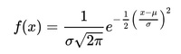
Where x is a normal random variable, μ is the mean, σ is the standard deviation, π is approximately 3.14159, and e is approximately 2.71828.

The random variable x in the normal equation is called the normal random variable. The normal equation is the probability density function (pdf) for normal distribution.

The Normal Curve

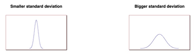
The graph of the normal distribution depends on two factors – the mean and the standard deviation. The mean of the distribution determines the location of the centre of the graph, and the standard deviation determines the height and width of the graph. When the standard deviation is large, the curve is short and wide; when the standard deviation is small, the curve is tall and narrow. All normal distributions look like a symmetric, bell-shaped curve, as shown below:

Probability and the Normal Curve

The normal distribution is a continuous probability distribution. This has several implications for probability.

• The total area under the normal curve is equal to 1.
• The probability that a normal random variable X equals any particular value is 0.
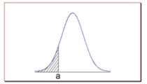
• The probability that X is greater than a equals the area under the normal curve bounded by a and plus infinity (as indicated by the non-shaded area in the figure below).
• The probability that X is less than a equals the area under the normal curve bounded by a and minus infinity (as indicated by the shaded area in the figure below).

Additionally, every normal curve (regardless of its mean or standard deviation) conforms to the following “rule”:

• About 68% of the area under the curve falls within 1 standard deviation of the mean.
• About 95% of the area under the curve falls within 2 standard deviation of the mean.
• About 99.7% of the area under the curve falls within 3 standard deviation of the mean.

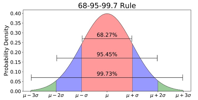
Collectively, these points are known as the empirical rule or the 68-95-99.7 rule. Clearly, given a normal distribution, most outcomes will be within 3 standard deviations of the mean.

Cumulative Distribution function

The cumulative distribution function () describes probabilities for a random variable to fall in the intervals of the form. The standard normal distribution is denoted with the capital Greek letter (phi), and can be computed as an integral of the probability density function:

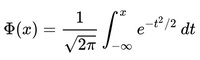
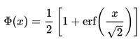
This integral can only be expressed in terms of a special function, called the error function. The numerical methods for calculation of the standard normal  are discussed below. For a generic normal random variable with mean  and variance, the  will be equal to:

The complement of the standard normal cdf, Q(x)=1- Φ(x), is referred to as the Q-function, especially in engineering texts. This represents the tail probability of the Gaussian distribution that is the probability that a standard normal random variable X is greater than the number x.

Properties:

• The standard normal cdf is 2-fold rotationally symmetric around (0,1/2): Φ(-x)=1-Φ(x).
• The derivative of Φ(x) is equal to the standard normal pdf ϕ(x): Φ'(x) = ϕ(x).
• The anti-derivative of Φ(x) is: ∫Φ(x) dx = x Φ(x) + ϕ(x).

Example

To Be Added

References & Resources

• Wikipedia