Introduction

In this section, we will discuss the shape of Binomial Distribution, and take a look at how they change as we tweak some of its paramaters, such as the number of trials or the probability of success. We will also talk about the fact that when the number of trials increases, the shape of the Binomial actually starts looking closer and closer to a full Normal Distribution. So, for such situations, we are going to use methods we've learned to calculate Normal Probability to approximate Binomial Probabilities.

The Shape of Binomial Distribution

Suppose we have a binomial random variable with the probability of success is 0.25 (25%).

This is what the distribution looks like when n = 10.

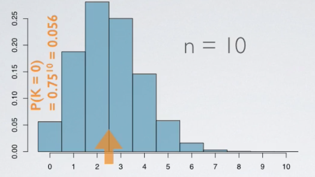
• Each bar represents a potential outcome.
• With 10 trials, the number of successes could range anywhere from 0 to 10 and therefore we have 11 bar here.
• Height of the bars represents the likelihood of these outcomes. For example, the probability of zero successes can be calculated as ten failures = 0.75¹⁰ = 0.056, which is the height of this bar.

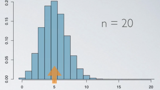
When n = 20, we see a change in the center of the distribution, which is expected since n × p is now different. The distribution is looking much less skewed.

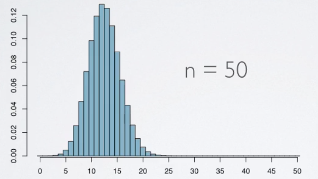
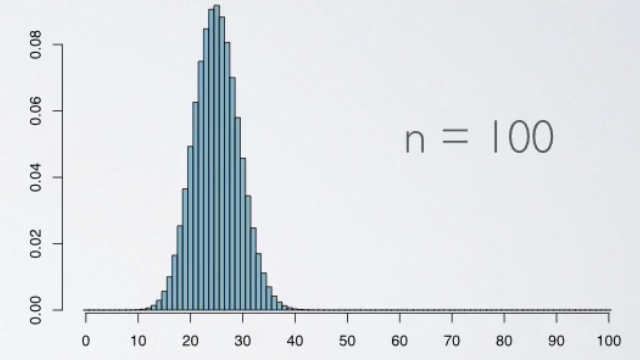
Increasing the sample size further to 50, the distribution looks even more symetric, and much smoother, and increasing the size even further to 100, the distribution looks no different than the normal distribution.

Normal Approximation to Binomial

The rule of thumb is the success-failure condition.

Success-failure rule: 
A binomial distribution meet the following conditions closely following a normal distribution. 

• np ≥ 10: at least 10 expected successes;
• n(1-p) ≥ 10: 10 expected failures;

And in cases where it does we can approximate the binomial distribution with the normal, where the parameters of the normal distribution are calculated as the mean and standard deviation of the binomial.

Binomial(n, p) ~ Normal(μ, σ)
where μ = np and σ = sqrt(np(1 - p))

In addition, there is a 0.5 adjustment to make the probabilities calculated the exact probabilities from the binomial distribution.

Example

We know that it must meet the following conditions:

n × 0.25 ≥ 10
and 
n × (1 - 0.25) ≥ 10

So, for both above, we need to find the maximum of n since that is going to be the minimum requried sample size. Then, we found n ≥ 40, that is we need the sample size n at least 40

References & Resources

• N/A