Introduction

The joint probability distribution for X and Y defines the probability of events defined in terms of both X and Y. As defined in the form below:

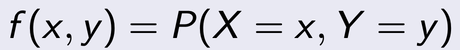
where by the above represents the probability that event x and y occur at the same time.

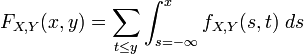
The cumulative distribution function for a joint probability distribution is given by:

In the case of only two random variables, this is called a bivariate distribution, but the concept generalises to any number of random variables, giving a multivariate distribution. The equation for joint probability is different for both dependent and independent events.

Discrete Case

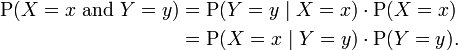
The joint probability function of two discrete random variables is equal to (Similar to Bayes' theorem):

In general, the joint probability distribution of n discrete random variables X₁ , X₂ , ... ,X_n is equal to:

This identity is known as the chain rule of probability.

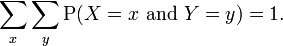
Since these are probabilities, we have:

generalising for n discrete random variables X₁ , X₂ , ... ,X_n :

Continuous Case

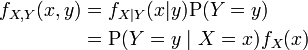
Similarly for continuous random variables, the joint probability density function can be written as f_X,Y(x, y) and this is :

where f_Y|X(y|x) and f_X|Y(x|y) give the conditional distributions of Y given X=x and of X given Y=y respectively, and f_X(x) and f_Y(y) give the marginal distributions for X and Y respectively.

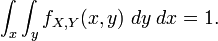
Again, since these are probability distributions, one has:

Mixed Case

In some situations X is continuous but Y is discrete. For example, in a logistic regression, one may wish to predict the probability of a binary outcome Y conditional on the value of a continuously distributed X. In this case, (X, Y) has neither a probability density function nor a probability mass function in the sense of the terms given above. On the other hand, a "mixed joint density" can be defined in either of two ways:

Formally, f_X,Y(x , y) is the probability density function of (X, Y) with respect to the product measure on the respective supports of X and Y. Either of these two decompositions can then be used to recover the joint cumulative distribution function:

The definition generalises to a mixture of arbitrary numbers of discrete and continuous random variables.

References & Resources

• N/A