Introduction

The next application that we’ll take a look at in this section is an important application that is used in many areas. If you’ve been following along in the section to this point it’s quite possible that you’ve gotten the impression that many of the applications that we’ve looked at are just made up by us to make you work. This is unfortunate because all of the applications that we’ve looked at to this point are real applications that really are used in real situations. The problem is often that in order to work more meaningful examples of the applications we would need more knowledge than we generally have about the science and/or physics behind the problem. Without that knowledge we’re stuck doing some fairly simplistic examples that often don’t seem very realistic at all and that makes it hard to understand that the application we’re looking at is a real application.

That is going to change in this section. This is an application that we can all understand and we can all understand needs to be done on occasion even if we don’t understand the physics/science behind an actual application.

In this section we are going to look at a method for approximating solutions to equations. We all know that equations need to be solved on occasion and in fact we’ve solved quite a few equations ourselves to this point. In all the examples we’ve looked at to this point we were able to actually find the solutions, but it’s not always possible to do that exactly and/or do the work by hand. That is where this application comes into play. So, let’s see what this application is all about.

Let’s suppose that we want to approximate the solution to f(x)=0 and let’s also suppose that we have somehow found an initial approximation to this solution say, x₀. This initial approximation is probably not all that good and so we’d like to find a better approximation. This is easy enough to do. First we will get the tangent line to at x₀ (Note: According to Taylor Series).

Now, take a look at the graph below.

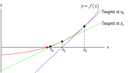
The blue line (if you’re reading this in color anyway…) is the tangent line at x₀. We can see that this line will cross the x-axis much closer to the actual solution to the equation than x₀ does. Let’s call this point where the tangent at x₀ crosses the x-axis x₁ and we’ll use this point as our new approximation to the solution.

So, how do we find this point? Well we know it’s coordinates, (x₁, 0), and we know that it’s on the tangent line so plug this point into the tangent line and solve for x₁ as follows,

So, we can find the new approximation provided the derivative isn’t zero at the original approximation.

Now we repeat the whole process to find an even better approximation. We form up the tangent line to f(x) at x₁ and use its root, which we’ll call x₂, as a new approximation to the actual solution. If we do this we will arrive at the following formula.

This point is also shown on the graph above and we can see from this graph that if we continue following this process will get a sequence of numbers that are getting very close the actual solution. This process is called Newton’s Method.

Here is the general Newton’s Method

Newton’s Method

If xn is an approximation a solution of and if the next approximation is given by,

This should lead to the question of when do we stop? How many times do we go through this process? One of the more common stopping points in the process is to continue until two successive approximations agree to a given number of decimal places.

Before working any examples we should address two issues. First, we really do need to be solving f(x)=0 in order for Newton’s Method to be applied. This isn’t really all that much of an issue but we do need to make sure that the equation is in this form prior to using the method.

Secondly, we do need to somehow get our hands on an initial approximation to the solution (i.e. we need x₀ somehow). One of the more common ways of getting our hands on x₀ is to sketch the graph of the function and use that to get an estimate of the solution which we then use as x₀. Another common method is if we know that there is a solution to a function in an interval then we can use the midpoint of the interval as x₀.

Let’s work an example of Newton’s Method.

Example 1

Use Newton's Method to determine an approximation to the solution to cosx = x that lies in the interval [0,2]. Find the approximation to six decimal places. Solution First note that we weren’t given an initial guess. We were however, given an interval in which to look. We will use this to get our initial guess. As noted above the general rule of thumb in these cases is to take the initial approximation to be the midpoint of the interval. So, we’ll use x0=1 as our initial guess. Next, recall that we must have the function in the form f(x)=0. Therefore, we first rewrite the equation as, We can now write down the general formula for Newton’s Method. Doing this will often simplify up the work a little so it’s generally not a bad idea to do this. Let’s now get the first approximation. At this point we should point out that the phrase “six decimal places” does not mean just get x1 to six decimal places and then stop. Instead it means that we continue until two successive approximations agree to six decimal places. Given that stopping condition we clearly need to go at least one step farther. Alright, we’re making progress. We’ve got the approximation to 1 decimal place. Let’s do another one, leaving the details of the computation to you. We’ve got it to three decimal places. We’ll need another one. And now we’ve got two approximations that agree to 9 decimal places and so we can stop. We will assume that the solution is approximately x4=0.7390851332.

In this last example we saw that we didn’t have to do too many computations in order for Newton’s Method to give us an approximation in the desired range of accuracy. This will not always be the case. Sometimes it will take many iterations through the process to get to the desired accuracy and on occasion it can fail completely.

The following example is a little silly but it makes the point about the method failing.

Example 2

Use x0=1 to find the approximation to the solution to Solution Yes, it’s a silly example. Clearly the solution is x=0, but it does make a very important point. Let’s get the general formula for Newton’s method. In fact we don’t really need to do any computations here. These computations get farther and farther away from the solution, x=0, with each iteration. Here are a couple of computations to make the point. So, in this case the method fails and fails spectacularly.

So, we need to be a little careful with Newton’s method. It will usually quickly find an approximation to an equation. However, there are times when it will take a lot of work or when it won’t work at all.

References & Resources

• http://tutorial.math.lamar.edu/Classes/CalcI/NewtonsMethod.aspx