Introduction

In this tutorial, we will play a game to introduce a Bayesian approach to inference. Throughout this tutorial, we will be making use of Bayes' theorem, properties of conditional probabilities, and probabilities tree.

The Game

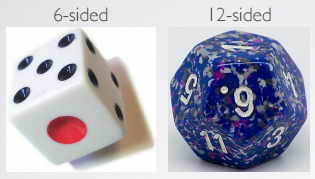
I have a die in each hand. One is a 6-sided die and the other is a 12-sided die:

Here are two questions:

• What is the probability of rolling ≥ 4 with a 6-sided die?
  Answer: the sample space, s = {1,2,3,4,5,6} and the interests are {4,5,6} out of the six, so

  P(≥4) = 3/6 = 1/2 = 0.5.

• What is the probability of rolling ≥ 4 with a 12-sided die?
  Answer: the sample space, s = {1,2,3,4,5,6,7,8,9,10,11,12} and the interests are {4,5,6,7,8,9,10,11,12} out of the twelve, so

  P(≥4) = 8/12 = 3/4 = 0.75.

For the goal is to roll ≥4, the 12-sided die is of course the good die because its probability is 75%.

Rules

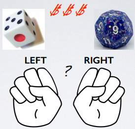
I have 2 dice, one 6-sided and the other 12-sided. I keep one die in left hand and the other in the right. But we don't know which die I'm holding in which hand. You pick a hand, left or right, I roll it. And I tell you if the outcome is ≥ 4 or not. I won't tell you what the outcome actually is. Based on this information you make a decision as to which hand holds the good, the 12-sided die. You could also choose to try again, in other words, collect more data. But each round costs you money. So you don't want to keep trying too many times.

This is a game and we made up some rules, but if you think about data collection, it is always costly. We love large sample sizes, it takes a huge amount of resources to obtain such samples. So the rules we are imposing aren't haphazardly made up, and they reflect some reality about conducting scientific studies.

Hypothesis and Decision

Let's first evaluate the possible decisions we might make.

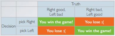
There are two possibilities for the truth. Either the good die is in the right hand or the good die is in the left hand.

The four possible outcomes are:

• If you guesssed that the right hand is holding the good die, and the good die is indeed on the right, then you win the game.
• If the good die is on the left but you picked right, you lose the game.
• Similary, if you picked left and the good die is on the right, then you lose.
• If you picked right and the good die is on the right, then you win.

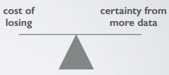
To avoid losing the game, you might want to collect as much data as possible, but that is costly as mentioned before!! So at some point before you are entirely sure, you have to just go ahead and make a guess. However, losing game also cost you, so there is a need to balance the cost associated with making the wrong decision and losing the game, against the certainty that comes with additional data collection.

Prior probabilities before collecting data

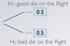
Question: Before we collect any data, you have no idea if I am holding the good die (12-sided) on the right hand or the left hand. Then, the probabilities associated with the following Hypothesis are:

P(H1: good die on the Right)	P(H2: good die on the left)
50% (0.5)	50% (0.5)

Above are the Prior Probability for the two competing claims, the two competing hypothesis. These probabilities represent what you believe before seeing any data. You could have conceivably made up these probabilities, but instead, we have chosen to make an educated guess.

Data Collection

Round 1

You pick the right hand for the 1st round, and you roll a number ≥ 4. Having observed this data point, the probabilities for the hypothesis are changed to:

P(H1: good die on the Right)	P(H2: good die on the left)
more than 50% (0.5)	less than 50% (0.5)

Actually Calculate the Probability

We started with two hypothesis, good die is on the right or the bad die is on the right. Initially, we have given these equal chances before actually get started with the data collection. These values are Prior Probability.

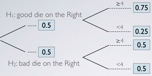
Then, in the data collection stage,

• If it is true that the good die is on the right, the probability of rolling a number ≥ 4 is going to be 75%. Complement of that, rolling a number < 4 is going to be 25%.
• If on the other hand, you are actually holding the bad die on the right, and you are picking the right hand. The probability of rolling a number ≥ 4 is 50%, and the complement, rolling a number < 4, is also 50%.

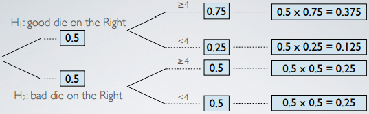
In the probability tree, the next step is to calculate the joint probabilities. So we multiply across the branches:

• There is a 37.5% chances that good die is on the Right and you roll a number ≥ 4.
• There is a 12.5% chances that good die is on the Right and you roll a number < 4.
• There is a 25% chances that the bad die is on the Right and you roll a number ≥ 4.
• There is a 25% chances that the bad die is on the Right and you roll a number < 4.

As we said, we did indeed roll a number > 4, so these are the 2 outcomes that we are most interested in:

• The top branch
• The third branch

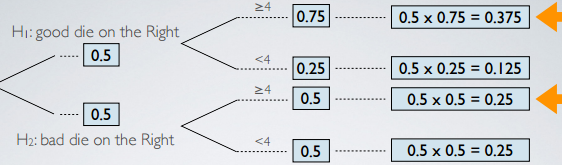
So what is the probability changes to the hypothesis? The probability could formally be written as:

P (H1: good die on the Right | You rolled ≥ 4 with the die on the Right )

This is a conditional probability, so we can make use of the Bayes theorem:

P (H1: good die on the Right | You rolled ≥ 4 with the die on the Right )
 
 
  P(Good die on the Right & Rolled ≥ 4 Right) 
= ----------------------------- 
      P(Rolled ≥4 Right)
 
 
      0.375
= ------------   = 60%
   0.375 + 0.25

The result come out to be 60%, so we can indeed see an increase up to 60%.

In the next roll

In the next roll, we get to take advantage of what we learned from the data. In other words, we update our prior with our Posterior probability from the previous iteration.

P(H1: good die on the Right)	P(H2: good die on the left)
0.6	0.4 (The compliment of 0.6)

Posterior Probability

The probability we just calculated is also called the Posterior probability. The Posterior probability is generally defined as P(hypothesis | data). It tells us the probability of a hypothesis we set forth, given the data we just observed.

The Posterior probability is different from P(data | hypothesis), also called a p-value, the probability of observed or more extreme data given the null hypothesis being true.

Reference & Resources

• N/A