Working with the binomial distribution
Example 1
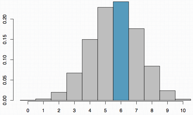
According to a 2014 Gallup poll, 56% of uninsured Americans who plan to get health insurance say they will do so through a government health insurance exchange. What is the probability that in random sample of 10 people exactly 6 plan to get health insurance through a government health insurance exchange?
Solution 1 - Use web app
The app link is available from https://gallery.shinyapps.io/dist_calc/
Solution 2 - Use R dbinom()
Alternatively, using R dbinom() function, we set the number of successes, the first argument to 6, the size to 10 and the probability of success to 0.56, and obtain the same answer 24.3%.
> dbinom(6, size = 10, p = 0.56)
 [1] 0.243
Solution 3 - Calculate by hand
We are looking for the probability of exactly 6 successes in 10 trials.
P(k=6) =  (10 6) × 0.566 × 0.444

            10!
      = ---------- × 0.566 × 0.444
          6! × 4!

     = 210 × 0.566 × 0.444

     = 0.243
Example 2
What is the probability that in a random sample of 1000 people exactly 600 plan to get health insurance through a government health insurance exchange?
- (a) 0.243, same as P(k=6)
- (b) less than 0.243
- (c) more than 0.243
Solution 1 - use the law of large numbers
The probability of success is P = 0.56.
In example 1:
- The sample size is 10;
- The expected number of successes would be 10 × 0.56 = 5.6.
- The difference between the expected and the desired number is then would be Δ = 6 - 5.6 = 0.4;
In this example:
- The sameple size is 1000;
- The expected number of successes is 1000 × 0.56 = 560;
- The difference between the expected and the desired number is Δ = 600 - 560 = 40;
Here, the desired outcome is much farther than the expected outcome and based on the law of large numbers, obtaining 600 successes when the expected is 560 should be a much less likely outcome that obtaining 6 successes when the expected is 5.6. Therefore, the answer is something less than 0.243.
Solution 2 - use R
Alternatively, using R dbinom() function, we set the number of successes, the first argument to 600, the size to 1000 and the probability of success to 0.56, and obtain the same answer 24.3%.
> dbinom(600, size = 1000, p = 0.56)
 [1] 0.00098
Example 3
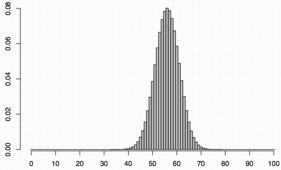
Describe the probability distribution of number of uninsured Americans who plan to get health insurance through a government health insurance exchange among a random sample of 100.
The probability of success is P = 0.56, as mentioned in Example 1. This time n = 100, this seems like a larger sample size. So let's see if it is actually large enough to yield a nearly normal distribution.
The rule is that we need at least 10 expected successes and 10 expected failures.
Success: np = 100 × 0.56 = 56 > 10
Fail: n(1-p) = 100 × 0.44 = 44 > 10
Therefore, we know the shape of this distribution will be nearly normal. Normal distribution has two parameters, mean and standard deviation. So to fully describe the distribution, we need to calculate these parameters, which we know can be estimated by the binomial, mean and standard devition.
μ = 56
σ = sqrt(100 × 0.56 × 0.44) = 4.96

Example 4:
What is the probability that at least 60 out of a random sample of 100 uninsured Americans plan to get health insurance through a government health insurance exchange?
Solution 1 - Use web app
The app link is available from https://gallery.shinyapps.io/dist_calc/
Solution 2 - Use R dbinom() and sum()
Alternatively, using R dbinom() function to get the probability and sum() function to get the bunch of probabilities. We set the number of successes, the first argument to 60:100, the size to 100 and the probability of success to 0.56, and obtain the same answer 24.3%.
> sum(dbinom(60:100, size = 100, p = 0.56))
 [1] 0.241
Solution 3 - Work out using normal distribution
We can make use of the fact that the distribution is nearly normal, with mean 56 and standard deviation 4.96.
When finding normal probabilities, we calculate the z score as the observation.
      60 - 56
Z = ----------- = 0.81
        4.96
Next step is to find the probability of Z > 0.81 from the normal probability table, that is roughly 0.209.
P(Z > 0.81) = 0.209
Once again, this probability is a little lower than the probabilities we have calculated using the App and R. This discrepancy is mostly due to the fact that under the normal distribution, probability of exactly 60 successes is undefined. To account for that, we apply a 0.5 correction to the observation of interest, and can work through the problem.
      59.5 - 56
Z = ------------- = 0.71
        4.96
Then the updated probability is:
P(Z > 0.71) = 0.239
The result is much closer to the exact probability.
References & Resources;
- N/A
Latest Post
- Dependency injection
- Directives and Pipes
- Data binding
- HTTP Get vs. Post
- Node.js is everywhere
- MongoDB root user
- Combine JavaScript and CSS
- Inline Small JavaScript and CSS
- Minify JavaScript and CSS
- Defer Parsing of JavaScript
- Prefer Async Script Loading
- Components, Bootstrap and DOM
- What is HEAD in git?
- Show the changes in Git.
- What is AngularJS 2?
- Confidence Interval for a Population Mean
- Accuracy vs. Precision
- Sampling Distribution
- Working with the Normal Distribution
- Standardized score - Z score
- Percentile
- Evaluating the Normal Distribution
- What is Nodejs? Advantages and disadvantage?
- How do I debug Nodejs applications?
- Sync directory search using fs.readdirSync